UNET CT Scan Segmentation using TensorFlow 2
preview version - final version coming soon
TL;DR;
This is a quick tour over Tensorflow 2 features and an UNET implementation using its framework and data pipeline.
I will make the notebook available on github available, after some clean up. But I am pre-publishing this for reference because I do not know when I will have time to make the source prettier.
Here is github source and results:
github.com/fsan/UNET_Remake
Let’s go
Migrating from TF 1.x to 2.x was not as easy as I thought it would be. But certainly not because of TF2. There are lots of perks and tricks you have to learn to use TF1 and they are necessary anymore. So at first you get stuck and starting thinking where you should put all that boilerplate code from before. In the end, it is much easier to learn TF2 from scratch than trying to adapt every TF1 concept you learned in the past.
So to explore some useful tools from TensorFlow and share some of what I learned I remade the content from one of my previous posts from 2018.
By that time, I was far less concerned about using the framework properly and its tools for a single pipeline than now. The main focus at that time was to implement the model from Ronneberger et al and get it working.
It was something I’ve done in a single night and by wrote that medium post next day. By consequence I hadn’t explorer many useful tools and concepts. This was not such a big problem at that time, but some people could reproduce the results and other not. And my best guess was that people could not reproduce the same procedures I did to preprocess and organize images. And even if I tried, probably I could not, because I hadn’t take any note and just relied on my memory to describe people.
I was very happy to see that many people got it working and made it much more useful than I though, such as estimating rooftop areas for solar policy by Britanny Bennet .
I do not intend to repeat myself in this post, and theory is better detailed in the original post. I will, in the next sections, explore some more details and concepts and I did not cover before and may be relevant for refreshing and ideas for this post.
I will be using the same IRCAD dataset again and will try to get same results from before.
There is a way of downloading the dataset, but YOU MUST check the IRCAD page to understand licensing and distribuition.
wget https://www.ircad.fr/softwares/3Dircadb/3Dircadb1/3Dircadb1.zip
unzip 3Dircadb1.zip; cd 3Dircadb1
for a in $(find . -name '*.zip'); do
    dx=$(dirname $a);
    fx=$(basename $a);
    echo $fx; echo $dx ;
        pushd $dx;
        unzip $fx;
    popd ; done
I will not strive for a very different implementation of the model, nor any different techniques I used by that time. Some code will be different from previous implementation because (1) I will be using TF2 pipeline as much as I can and (2) I learned other things that may helped me to make things simpler.
Computed Tomography Scan
CT Scans are medical images produced by the combination of many measurements done simultaneously. For newbies in the matter like me, all the physics and math behind it are almost magic, and it is indeed one of the most complex piece of equipment built by humanity until this day. Some references how it works here.
But in a very simplified way, this equipment is capable of generating 3D images from inside the body and determining density properties at each point given its own resolution capability. This 3D images can be sliced in 2D portions to show a cross section of interest for medical analysis and are used most of the time to aid on medical diagnostics.
Source: Medical News Today
DICOM
The DICOM is a standard format for medical images and is the format used in the dataset chosen for this experiment. It is the most common format to find medical image data and tensorflow-addons package now allows you to load and integrate with tensorflow.image package easily.
Reading DICOM files in TensorFlow
Reading DICOM files in TF2 does not require any external packages anymore. This is great, because reading it as tensors and processing in the same pipeline makes everything easier to integrate and faster to execute. Reading a DICOM file goes in 2 steps. 1. Reading the binary file 1. Converting from DICOM to Image
def process_path(filename):
    image_bytes = tf.io.read_file(filename)
    image_data = tfio.image.decode_dicom_image(image_bytes,
                                               scale='auto',
                                               on_error='lossy',
                                               dtype=tf.uint8 )
For more information about reading DICOM files directly check this official guide.
TensorFlow Dataset
A TensorFlow Dataset is a pretty useful concept to load, process and feed your model. It allows you to create a functional-like pipeline where you filter and map functions to data as they pass through the pipeline. It also allows you to cache data for more speed, shuffle and repeat to feed your model.
For more information on TF datasets check this link.
import pathlib
root_dir = pathlib.Path(r"D:\data\3Dircadb1")
all_dataset = tf.data.Dataset.list_files(str(root_dir/'*/PATIENT_DICOM/*'))
D = 256 # image side size we will be using

def process_path(filename):
    patient_bytes = tf.io.read_file(filename)
    patient_image = tfio.image.decode_dicom_image(patient_bytes,
                                                  scale='auto',
                                                  on_error='lossy',
                                                  dtype=tf.uint8)
    patient_image = tf.squeeze(patient_image, axis=0)
    # normalize between 0. and 1.
    patient_image = tf.image.convert_image_dtype(patient_image, tf.float32)
    patient_image = tf.image.resize(patient_image, (D,D))

    mask_path = tf.strings.regex_replace(filename,
                                         'PATIENT_DICOM',
                                         'MASKS_DICOM/liver/')

    mask_bytes = tf.io.read_image(mask_path)
    mask_image = tfio.image.decode_dicom_image(mask_bytes,
                                               on_error='lossy',
                                               dtype=tf.uint8)

    # need to squeeze, because dicom are supposed to be 3D
    # but in this dataset, each dicom image is just one slice
    # (1, W, H, 1) -> (W, H, 1)

    mask_image = tf.squeeze(mask_image, axis=0)
    mask_image = tf.image.convert_image_dtype(mask_image, tf.float32)
    mask_image = tf.image.resize(mask_image, (D,D))

    return patient_image, mask_image
Filtering dataset
One good thing about using tf.datasets is to be able to setup your data processing pipeline. For example, in 3D-IRCARD dataset you may have problem training your model if there is some large amount of empty masks in proportion of non-empty. You may want to set them to similar sizes or to use just a small part of empty images for training the model. In the case of IRCAD, when training for some organs that only exist in one part of the body, the liver for example, you will find lots of empty images. It is nice to have empty images, because your model needs to differentiate what a not-liver is. But having too few blank images makes your model overfit always putting a liver format where it think it should be. It will be kind of right because livers have more or less the same size and shape, but it will miss terribly saying that you have a liver inside your lungs.
One way of filtering images is too remove randomly a certain amount to balance the amount of examples.
def remove_empty_mask_with_prob(mask, prob=.6, epsilon=1e-3):
    if tf.math.less_equal(tf.math.reduce_sum(mask),
                          tf.cast(epsilon, tf.float32)):
        return tf.math.greater(
            tf.cast(tf.squeeze(tf.random.uniform((1,))), tf.float32),
            tf.cast(prob, tf.float32))
    else:
        return True

def filter_dataset_fn(ds):
    return ds.filter(lambda _, y: remove_empty_mask_with_prob(y))

# ...

filtered_dataset = full_dataset.apply(lambda x: filter_dataset_fn(x))
Mapping
One common action when working with images, and many other datasets, is to process data and give the model something easier to digest or adding noise to the input so the model does not overfit due to some similarities. With TF Datasets it is possible to stack this operations like this:
@tf.function
def median_filter_with_prob(sample_pair, prob=1.):
    r = tf.cast(tf.squeeze(tf.random.uniform((1,))), tf.float32)
    if tf.math.less_equal(r,
                          tf.cast(prob, tf.float32)):
        return sample_pair[0], tfa.image.median_filter2d(sample_pair[1], filter_shape=(4,4))
    else:
        return sample_pair

def apply_random_median_filter(ds, prob=.5):
    return ds.map(lambda x, y: median_filter_with_prob((x,y), prob))

@tf.function
def gauss_noise_with_prob(sample_pair, expected_noise_rate=1e-2, prob=1.):
    r = tf.cast(tf.squeeze(tf.random.uniform((1,))), tf.float32)
    if tf.math.less_equal(r,
                          tf.cast(prob, tf.float32)):
        var = 1e-2
        mean, sigma = 0., tf.math.pow(var, 0.5)
        shape = (D, D, 1)
        noise = tf.random.normal(shape, mean, sigma) * expected_noise_rate
        noise_image = tf.math.add(sample_pair[0], noise)

        noise_image = tf.clip_by_value(noise_image, clip_value_min=0., clip_value_max=1.)
        return noise_image, sample_pair[1]
    else:
        return sample_pair

def apply_random_gauss_noise(ds, prob=.25):
    return ds.map(lambda x, y: gauss_noise_with_prob((x,y), prob))
And finally stack them to your data pipeline like:
train_dataset = dataset.apply(lambda x: apply_random_median_filter(x))
train_dataset = dataset.apply(lambda x: apply_random_gauss_noise(x))
To exhibit an image you can take it from your dataset
n =1
sample_images = list(train_dataset.skip(np.random.randint(0, train_size-n)).take(n))
for x in sample_images:
    patient = x[0].numpy()
    mask = x[1].numpy()

    fig, axes = plt.subplots(1,2, figsize=(8,8))
    axes[0].imshow(np.squeeze(patient), cmap='gray', interpolation='none', filternorm=False)
    axes[0].set_title('Patient Scan')
    axes[0].set_axis_off()
    axes[1].imshow(np.squeeze(mask), cmap='gray', interpolation='none', filternorm=False,
                  norm=plt.Normalize(vmin=0., vmax=1.))
    axes[1].set_title('Segmentation')
    axes[1].set_axis_off()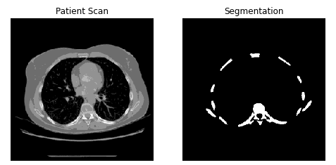
Modeling in TF2
You have basically 3 ways of modeling in TF2 using integrated keras.
- Sequential: You stack one layer in front of the other and use common model interface to train (fit) and evaluate your model.
- Functional: A functional-like API is provided so you can build your model much like building a graph
- Model Class Override: You can build your models overwriting default methods and basically applying any rule you like.
Overriding keras.Model to build a Custom Class is pretty useful for researchers who want to test new models or techniques and for treating special complex cases.
The UNET case is not complex, but for sake of learning and testing the concept I used it anyway. And using custom classes is almost as easy as using other methods:
The most basic of implementation demands you to override 2 methods: __init__ and call.
class YourCustomModel(tf.keras.Model):

    def __init__(self):
        super(UNET_Model, self).__init__()
        # ...

    def call(self):
        # ...
Callbacks
One thing I haven’t covered in the first article and it is actually pretty useful are TensorFlow Callbacks. Callbacks, as in any form of them in programming context, have an interface are injected in a framework/pipeline/code to execute user code in predetermined moments.
TensorFlow already have many useful callback function, but some of the more used are:
- ModelCheckpoint: Saves your model with certain periodicity. REFERENCE
- EarlyStopping: Automatically stops your model training if it does not improveDOCUMENTATION
- TensorBoard: reports the metrics and results of your model into a TensorBoard dashboard GUIDE
You can also implement your own CallBacks by just following Callbacks interface.
from tensorflow.keras.callbacks import ModelCheckpoint,
                                       EarlyStopping,
                                       TensorBoard

class UNET():
        def __init__(self,
                 optimizer,
                 loss,
                 metrics=[tf.keras.metrics.mean_squared_error],
                 num_epochs=150,
                 batch_size=32,
                 checkpoint_path="unet.ckpt"):

        self.model = UNET_Model()

        # ...

        self.checkpoint_cb = ModelCheckpoint(filepath=checkpoint_path,
                                             monitor='loss',
                                             save_best_only=False,
                                             save_weights_only=True,
                                             save_freq='epoch',
                                             verbose=1)

        self.early_stop_cb = EarlyStopping(monitor='loss',
                                       min_delta=5e-5,
                                       patience=5,
                                       verbose=1)

        self.tensorboard_cb = TensorBoard(log_dir='logs',
                                          histogram_freq=0,
                                          write_graph=True,
                                          write_images=True,
                                          update_freq='epoch',
                                          profile_batch=2,
                                          embeddings_freq=10)

        self.callbacks = [
                        self.checkpoint_cb,
                        self.early_stop_cb,
                        self.tensorboard_cb
                         ]

        self.model.compile(optimizer=self.optimizer,
                           loss=self.loss_function,
                           metrics=self.metrics)

        # ...
I won’t explain how each one of this callbacks work because their documentation is actually very small and simple, and in the end I would just be paraphrasing what is written there.
Metrics
Metrics in TF are just values that you can use keep track during training but do not influence training.
For example, you may use Dice score to train, and if you find necessary keep track of mean_squared_difference or any other value.
I also will not go over metrics, because it is very well documented and explained here.
UNET Model
Just to refresh the idea of UNET model, it goes like this:
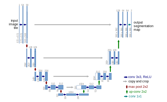 Source: Ronnenberger et al, 2015
In UNET the basic idea is to feed an image and minimize the output difference to a segmentation image. So the input and output of the model are images.
Loss function
For the model to learn what are the important features to observe, first it is necessary to tell it how to compare segmentation images.
Segmentation images, when only considering one class for segmentation, are binary. This means, that they are either 0 where there is no mask, and 1 where the mask is selecting the object of interest.
Simple metrics like mean_squared_difference are no good for cases like this, because the fastest route to minimize differences is to go to the mean value all around the image.
So people have used some different methods:
- Accuracy
- Jaccard Index (Intersection Over Union)
- Dice-Sorosen Coefficient
I will not explain each one of them, I already did some explanation in previous post but you can get a very nice visualization in this Ekin Tiu post. But for segmentation, usually Dice (f1-score) is good because it provides an positive increase releation of intersection area over the false positive and negative detections.
The loss function using dice can be computed as the negative of its value. So when we minimize the loss, we increase the Dice Score.
The single class dice function can be computed as:
from tensorflow.keras import backend as K

def dice_coef(y_true, y_pred, smooth = 1.):
    y_true_f = K.flatten(y_true)
    y_pred_f = K.flatten(y_pred)
    intersection = K.sum(y_true_f * y_pred_f)
    return (2. * intersection + smooth) / (K.sum(y_true_f) + K.sum(y_pred_f) + smooth)

def dice_coef_loss(y_true, y_pred):
    return -dice_coef(y_true, y_pred)
Convolution and Deconvolution Layers
The main two types of structures in UNET helps to condense feature and then create the output. In a very brief way, if you need more details, please check my previous post, the UNET model create layers by convolving features and then create the output by “de-convolving” the data with adjusted weights.
Convolution Layer This will be just a very (VERY) simple explanetion. For more details, or a real explanation please check my other post.
The full structure is composed of 3 types of layers:
- Convolution Layer: capture features with locally dependency
- MaxPooling: Reduces dimensionality by capturing the biggest (or smallest) value in a region
- Dropout: Intended to help avoiding overfitting, it “forgets” the result some times.
def get_conv_layer(kernel_size, filter_size, pool_size, name):
    init = 'glorot_uniform'
    conv1   = tf.keras.layers.Conv2D(kernel_size, filter_size, activation='relu', padding='same', kernel_initializer=init ,name='conv2d_'+str(name)+'1')
    conv2   = tf.keras.layers.Conv2D(kernel_size, filter_size, activation='relu', padding='same', kernel_initializer=init, name='conv2d_'+str(name)+'2')
    maxpool = tf.keras.layers.MaxPooling2D(pool_size=pool_size, name='maxpool_'+str(name))
    dropout = tf.keras.layers.Dropout(0.5, name='dropout_'+str(name))
    return conv1, conv2, maxpool, dropout
Deconvolution Layer
The Deconv layer does the opposite. It will build step by step building up the result image.
In Convolution Layer, when running MaxPooling, the pool_size determines the area which will be summarized in one value.
In the Deconvolution Layer the concatenate and Conv2DTranspose helps rebuilding the data
def get_deconv_layer(kernel_size, filter_deconv_size, stride_size, filter_conv_size, name):
    init = 'glorot_uniform'
    deconv1 = tf.keras.layers.Conv2DTranspose(kernel_size, filter_deconv_size, strides=stride_size,
                                                activation='relu', padding='same', kernel_initializer=init, name='deconv2d_'+str(name)+'1')
    merge1 = tf.keras.layers.concatenate
    conv1 = tf.keras.layers.Conv2D(kernel_size, filter_conv_size, activation='relu', padding='same', kernel_initializer=init, name='deconv2d_'+str(name)+'2')
    conv2 = tf.keras.layers.Conv2D(kernel_size, filter_conv_size, activation='relu', padding='same', kernel_initializer=init, name='deconv2d_'+str(name)+'3')

    return deconv1, merge1, conv1, conv2
Calling the layers
This post is alredy getting pretty large and I haven’t even show the results or argued about it. So I won’t be talking about the source code itself, as it is available on the github in the link in the beginning of the post. But I will let part of the code for building the conv and deconv layers here. But rest assured, only thing being done is to follow the UNET architecture, only resizing in something that fits in my computer.
Convolution Layer
def call_conv_layer(inputs, conv1, conv2, maxpool, dropout):
    c1 = conv1(inputs)
    c1 = conv2(c1)
    mp = maxpool(c1)
    dp = dropout(mp)

    return c1, dp
Deconvolution Layer
def call_deconv_layer(inputs_1, inputs_2, deconv, merge, conv1, conv2):
    up = merge([deconv(inputs_1), inputs_2], axis=3)
    cv = conv1(up)
    cv = conv2(cv)

    return cv
Putting all together
- Input -> Conv Layer 1 -> Conv Layer 2 … ->
- Midle Convution2D layers ->
- Deconv Layer 1 -> Deconv Layer 2 -> …
- Output Layer
ip = self.input_layer(inputs)

c1, d1 = call_conv_layer(ip, self.conv2d_11, self.conv2d_12, self.maxpool_1, self.dropout_1)
c2, d2 = call_conv_layer(d1, self.conv2d_21, self.conv2d_22, self.maxpool_2, self.dropout_2)
# ...
c9 = self.conv2d_51(d6)
c10 = self.conv2d_52(c9)
# ...
c13 = call_deconv_layer(c10, c6, self.deconv2d_131, self.merge_13, self.conv2d_131, self.conv2d_132)
c14 = call_deconv_layer(c13, c5, self.deconv2d_141, self.merge_14, self.conv2d_141, self.conv2d_142)
# ...
z = self.output_layer(c18)
return z